Audio generation using Language Models
What is a language model?
Language models — like ChatGPT, Llama and Mistral — are a hot topic nowadays and everybody seem to be trying them out; but, what about language models for audio generation? In this article, I’ll show you some of the experiments I did to generate audio using GPT2, EnCodec and EnCodecMAE. But first, let’s talk about language models (LMs).
Language models estimate probabilities of sequences of words given a corpus. So, what’s the probability of a sequence? Given a sequence of length : , its probability is calculated as the joint probability of every element in the sequence: Using the chain rule of probability, and assuming an ordering of the elements, it can be expressed as: Let’s explain this with a concrete example. Let’s say we have the following sentence:
"I play football"
The first step is to turn this sentence into a sequence. There are many possible ways to do it:
"[I, play, football]"
or
"[I, play, foot#, #ball]"
or
"[I, ,p,l,a,y, ,f,o,o,t,b,a,l,l]"
Tokenization is the process of turning a corpus into sequences of symbols. The symbols could be words like in the first example; or allow subwords like decomposing football in foot and ball; or could be chars like in the last example.
Let’s stick with the first example of tokenization and calculate the probability of the sentence. According to the rule of chain we have
Each term in the equation tells us the probability of a word given the previous words. If we train a neural network to predict the next word given the previous ones, and we use cross-entropy as loss function, then the outputs will correspond to each of the terms in the equation. The important detail is that our models have to be unable to ‘see’ into the future; if we peek into the future, then the probabilities will no longer be only conditioned in the past elements of the sequence. For recurrent neural networks this restriction is inherent to the model as tokens are processed in the sequence order. In the case of transformers, attention is computed between each query and only the past key-values by using attention masks. Pre-deep learning methods, like n-grams, would assume that the current output only depends on the previous n-1 outputs. Also causal convolutional neural networks, like Wavenet (Oord et al., 2016), can be used as language models, and the receptive field would be the equivalent to the n in n-grams.
Audio tokenization
The idea explained in the above section can be extended to model any sequence, not only text. Let’s try to use it for audio! The first step is to turn the audio into a sequence , as we did with the sentence. Audio itself is a sequence of discrete values, where the sampling rate defines how many values there are in 1 second. For speech, a common value is 16000 Hz, and for music 44100 Hz. This means that if we have 1 second of music and want to predict the next sample, the model will have to take the 44100 previous values into account. That’s really hard and computationally expensive, specially for recurrent neural networks (RNN) and transformers, which are the 2 leading models for sequence modelling in NLP. One workaround is to learn a more compact representation of audio. We will take a look into EnCodec (Défossez, Copet, Synnaeve & Adi, 2022), a neural audio codec from Meta, which uses a deep neural network to compress 1 second of audio into a sequence of only 75 elements.
EnCodec
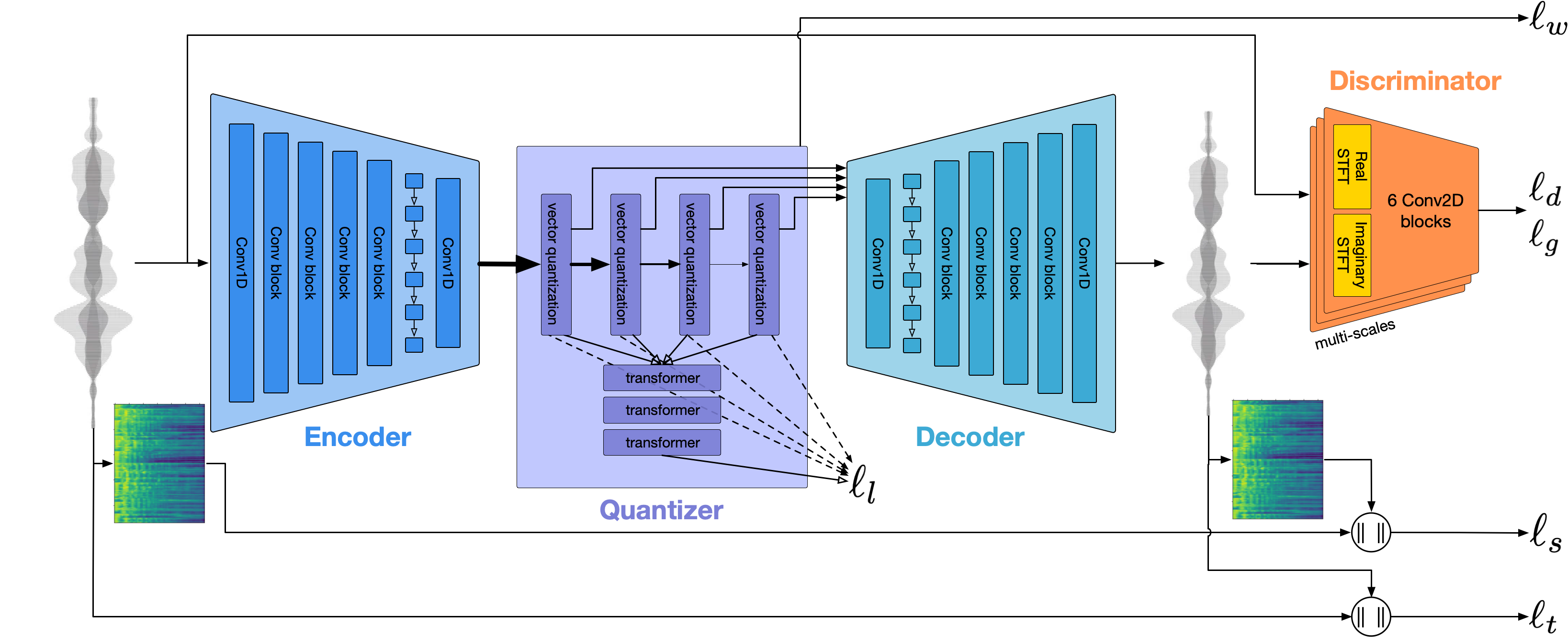
EnCodec architecture. From (Défossez, Copet, Synnaeve & Adi, 2022)
To further reduce the size of the waveform, EnCodec quantizes the bottleneck. The idea is that a quantization layer will map each of these 128-D vectors into one of 1024 possible integers. This is done by learning a codebook, which is just a lookup table with 1024 128D vectors (codes). Then, during inference, the output of the encoder is compared against each of the codes and the index corresponding to the closest one is returned. 1024 possible values can be represented using 10 bits. This means that 1 second of audio could be represented as a sequence of 75 10 bits elements, which gives a bitrate of 750 bits per second (bps). Our original audio had a sampling rate of 24000 Hz with 16 bit depth. That means 24000*16 bits per second, which is 384 Kbps. With this quantization we would be achieving a reduction of 512 in size! However there is a problem: the quality of the compressed audio will be very bad.
To solve this problem, EnCodec uses a residual vector quantizer (RVQ), which means that the residual between the encoder output and the closest code of the first quantizer is then quantized by the second quantizer. This allows to use multiple quantizers that refine the outputs of the previous quantizers. If we use 8 quantizers, we can get a decent audio quality and would be representing 1 second of audio with 8 sequences of 75 10 bits elements. That is 6 kbps and a reduction of 64 in size. Nice!
Now, let’s write some code in Python to tokenize audio using EnCodec:
from encodec import EncodecModel
import librosa
import torch

def tokenize(filename, model, sr=24000, num_quantizers=8):
    with torch.no_grad():
        x, fs = librosa.core.load(filename, sr=sr)
        codes = model.encode(torch.from_numpy(x)[None,None,:])[0][0]
    return codes

def detokenize(codes, model):
    with torch.no_grad():
        decoded_x = model.decode([(codes,None)])
    return decoded_x.detach().cpu().numpy()[0,0]

NUM_QUANTIZERS = 8

model = EncodecModel.encodec_model_24khz()
codes = tokenize('/mnt/hdd6T/jamendo/00/565800.mp3', model)
reconstruction_8q = detokenize(codes[:,:NUM_QUANTIZERS], model)
These are some audio samples of encoding/decoding the same audio with a different number of quantizers:
Multi-sequence patterns
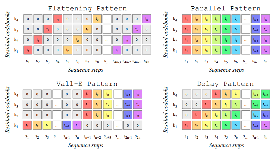
Codebook patterns. From (Copet et al., 2023)
- Flattening pattern: the idea is to interleave the sequences of length from each of the quantizers. Here is the element corresponding to the timestep and quantizer :
This pattern allows the model to predict the next element based in the previous quantizers outputs from the same timestep and all the outputs from previous timesteps. This way, the dependence between quantizers can be modelled. The drawback is that now the resulting sequence is times longer, making it computationally more expensive and harder to model.
Parallel pattern: this pattern is kind of opposite to the flattening one; the quantizers are assumed to be independent so in this pattern all the sequences are predicted in parallel. This approach doesn’t increase the sequence length but it might lead to worse results because of the independence assumption.
Vall-E pattern: this is the pattern used in Vall-E (Wang et al., 2023). In this pattern, the model will return the sequence corresponding to the first quantizer, and then the remaining quantizers in parallel. This means that the second to last quantizers are assumed to be dependent of the first quantizer, but independent between them. This can be considered a mid-point between the flattening and parallel patterns, as the sequence length will be , and the dependence between the first quantizer and the remaining ones is modelled. This approach makes sense as the first quantizer will be the one that reconstructs most of the signal while the following ones add detail.
Delay pattern: this is the pattern used by MusicGen (Copet et al., 2023). As in the parallel and Vall-E pattern, multiple sequences are predicted in parallel. However, both the time and quantizer dependences are modelled, while the sequence length is not significantly increased. This is achieved by delaying by one each quantizer sequence. For example, let’s look at the figure and try to understand it:
- In the first step , only the output for the first tokenizer is generated.
- In the second step , we have access to the output of the first tokenizer in , so we can produce 2 more outputs: for quantizer , and for the second quantizer .
- In the third step , we have access to the 2 first timesteps of the first tokenizer and the first timestep of the second tokenizer. We can generate the third timestep of the first tokenizer, the second timestep of the second tokenizer, and the first timestep of the third tokenizer.
- And so on…
Now, let’s write the Python code to apply the delay pattern to the EnCodec codes and also to remove the delay:
def roll_along(arr, shifts, dim):
    #From: https://stackoverflow.com/a/76920720
    assert arr.ndim - 1 == shifts.ndim
    dim %= arr.ndim
    shape = (1,) * dim + (-1,) + (1,) * (arr.ndim - dim - 1)
    dim_indices = torch.arange(arr.shape[dim], device=arr.device).reshape(shape)
    indices = (dim_indices - shifts.unsqueeze(dim)) % arr.shape[dim]

    return torch.gather(arr, dim, indices)

def apply_delay_pattern(codes):
    codes = torch.nn.functional.pad(codes+1,(0,codes.shape[1]-1))
    codes = roll_along(codes, torch.arange(0,codes.shape[1], device=codes.device)[None,:].tile((codes.shape[0],1)), 2)
    return codes

def unapply_delay_pattern(codes):
    codes = roll_along(codes, -torch.arange(0,codes.shape[1], device=codes.device)[None,:].tile((codes.shape[0],1)), 2)
    codes = codes[:,:,:-codes.shape[1]]
    return codes
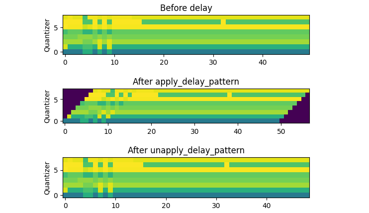
Result of applying the delay pattern
It can be seen that this approach adds only elements to the original sequence, which in this case is only 7 extra elements.
Turning GPT2 into an audio generator
GPT2 (Radford et al., 2019) is the predecessor of GPT3, and it’s actually a lot smaller so it can fit in a consumer-grade GPU. It’s basically a transformer with the causal attention mask that allows us to use it for language modelling. Using it in Python is very easy, thanks to HuggingFace transformers:
from transformers import GPT2Model

gpt = GPT2Model.from_pretrained('gpt2')
Adapting GPT2 to our inputs
We will have to make some modifications to this model to make it work with our inputs:
- The model has to predict as many outputs per timestep as quantizers. Each quantizer can have 1024 different values, and also can be empty because of the delay pattern. This means 1025 possible classes for each quantizer. We can make a linear output classifier with 1025*8 neurons and then reshape it as a tensor of probabilities with shape .
- The inputs to GPT2 can be discrete (corresponding to the units defined by its pretrained tokenizer), or continuous. When the input are discrete tokens, a lookup table is learned by the model to turn each token into a continuous vector. In our case it’s a bit more complicated as we have 8 discrete tokens per timestep. What we do is to learn a lookup table with 8*1025 possible values and map each quantizer value. Then, the 8 retrieved vectors are summed and used as the input to GPT2.
Prompting with EnCodecMAE
Also, we want to have some control over the generated audio at inference time. One way to achieve this is by prepending a prompt to the input tokens. The prompt could be a sequence of words describing the audio, an image, another audio, etc… I’ve been working in ways to represent audios recently, and proposed EnCodecMAE (Pepino, Riera & Ferrer, 2023), so I’ll use these audio vectors as prompt. EnCodecMAE is a general audio representation model, which is trained in a similar way to BERT. It was trained with a mixture of speech, music and general audio datasets. The discrete targets to reconstruct from the masked inputs were the EnCodec tokens of the unmasked audio.
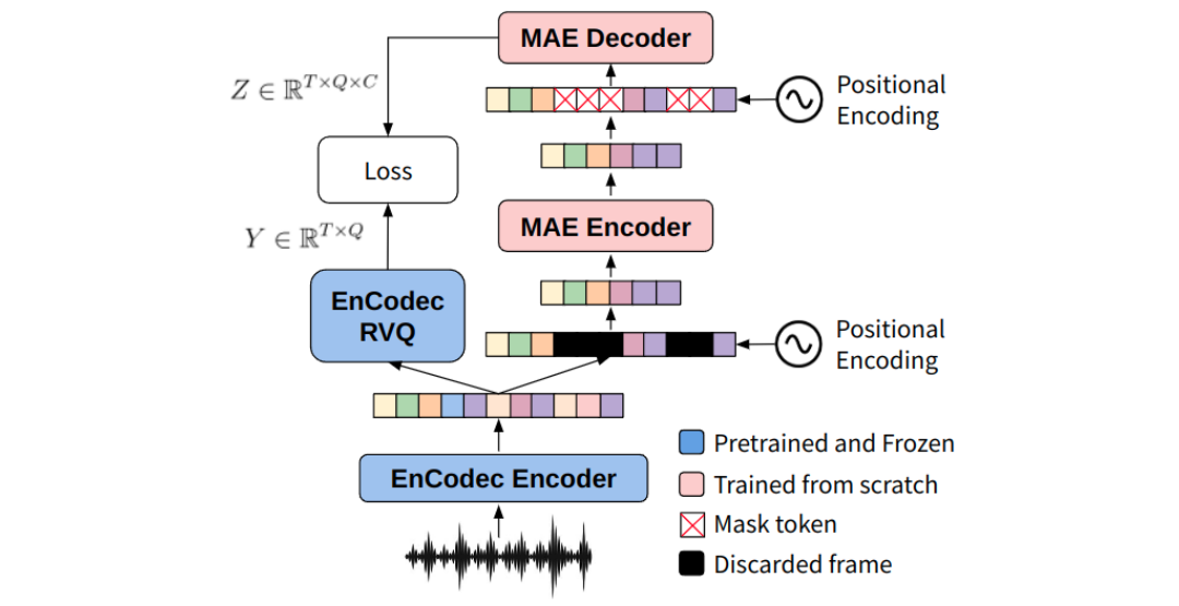
EnCodecMAE architecture. From (Pepino, Riera & Ferrer, 2023)
Putting everything together
Now, we can make a Pytorch Lightning module to encapsulate everything in a class:
import pytorch_lightning as pl

class EnCodecGPT(pl.LightningModule):
    def __init__(self, num_q=8, optimizer=None, lr_scheduler=None):
        super().__init__()
        self.encodec_model = EncodecModel.encodec_model_24khz()
        self.num_q = num_q
        self.num_codes = 1024
        self.vocab_size = self.num_q * (self.num_codes + 1)
        self.gpt = GPT2Model.from_pretrained('gpt2')
        self.vocab_embed = torch.nn.Embedding(self.vocab_size, self.gpt.embed_dim)
        self.classification_head = torch.nn.Linear(self.gpt.embed_dim, self.vocab_size)
        self.optimizer = optimizer
        self.lr_scheduler = lr_scheduler

    def forward(self, x, prompt=None):
        #Encodec tokens:
        with torch.no_grad():
            codes = self.encodec_model.encode(x)[0][0][:,:self.num_q]
        #Delay pattern:
        codes = apply_delay_pattern(codes)
        #Offset each quantizer by 1025 and pass through LUT:
        input_vocab_embed = torch.arange(self.num_q, device=x.device)[None,:,None]*(self.num_codes + 1) + codes
        gpt_in = self.vocab_embed(input_vocab_embed).sum(axis=1)
        #Prepend prompt:
        if prompt is not None:
            gpt_in = torch.cat([prompt[:,None,:],gpt_in],axis=1)
        #Pass through GPT:
        gpt_out = self.gpt(inputs_embeds = gpt_in)
        #Make classification:
        preds = self.classification_head(gpt_out['last_hidden_state'])
        preds = preds.view(preds.shape[0],preds.shape[1],self.num_q,self.num_codes+1)
        return preds, codes

    def training_step(self,x, batch_idx):
        wav = x['wav'].unsqueeze(1)
        preds, targets = self(wav, x['prompt'])
        preds = preds.transpose(1,3)[:,:,:,:-1]
        loss = torch.nn.functional.cross_entropy(preds, targets)
        self.log('train_loss', loss)
        return loss

    def validation_step(self,x, batch_idx):
        wav = x['wav'].unsqueeze(1)
        preds, targets = self(wav, x['prompt'])
        preds = preds.transpose(1,3)[:,:,:,:-1]
        loss = torch.nn.functional.cross_entropy(preds, targets)
        self.log('val_loss', loss)

    def configure_optimizers(self):
        opt = self.optimizer(self.trainer.model.parameters())

        if self.lr_scheduler is not None:
            if self.lr_scheduler.__name__ == 'SequentialLR':
                binds = gin.get_bindings('torch.optim.lr_scheduler.SequentialLR')
                lr_scheduler = self.lr_scheduler(opt, schedulers=[s(opt) for s in binds['schedulers']])
            else:
                lr_scheduler = self.lr_scheduler(opt) if self.lr_scheduler is not None else None
        else:
            lr_scheduler = None
        del self.optimizer
        del self.lr_scheduler
        opt_config = {'optimizer': opt}
        if lr_scheduler is not None:
            opt_config['lr_scheduler'] = {'scheduler': lr_scheduler,
                                          'interval': 'step',
                                          'frequency': 1}
        return opt_config
The full code for training can be found here.
Decoding audio
Autoregressive sampling
Once the model is trained, we want to generate audios with it. To sample from language models we have to do what is called autoregressive sampling.
- First, the prompt is fed to GPT2. An output is generated: this is the first sample generated by our model.
- We feed the prompt and the first sample generated by GPT2 and get the second sample.
- We keep repeating this process as long as we want, or until a special token (end of audio) is returned by the model.
A nice thing about HuggingFace GPT2 implementation is that it allows key-value caching. This means that we don’t need to generate all the intermediate outputs and compute attention with all the queries all the time during inference, as intermediate results are cached at each autoregressive sampling iteration. This saves a lot of computations reducing the time required to generate the sequences. This is not a minor detail as autoregressive sampling is expensive because it cannot be parallelized.
Different flavors of sampling
One very important detail to discuss is how to pass from probability outputs to an actual output generated by the language model. There are many approaches, and those are discussed in more depth here. Some options are:
- Greedy Search: The output is the token with highest probability (argmax).
- Sampling: The output is picked randomly following the distribution returned by the model. By dividing the logits by a scalar called temperature, if we make it lower than 1 we can make the distribution sharper (give more probability to the most probable tokens) or if we make it higher than 1 the distribution gets more flat. In the extreme, a temperature tending to 0 will be equivalent to greedy search, while a temperature tending to infinity will be like sampling from a uniform distribution. Temperature allows us to play with the generations, making them more diverse/random (higher temperature) or more stable (lower temperatures). Sometimes, the generations might get stuck in loops and increasing temperature can be a solution.
- Top-k Sampling: Before sampling, we can choose the k tokens with highest probability and redistribute the mass probability among them.
In the following Python snippet we will use temperature sampling:
def generate(prompt_filename, encodecmae, lm_model, temperature=1.0, generation_steps=300):
    prompt = encodecmae.extract_features_from_file(prompt_filename)
    prompt = prompt.mean(axis=0)
    with torch.no_grad():
        prompt = torch.from_numpy(prompt).to(lm_model.device)
        gpt_in = prompt.unsqueeze(0).unsqueeze(0)
        past_keys=None
        generation = []
        for i in tqdm(range(generation_steps)):
            outs = lm_model.gpt(inputs_embeds=gpt_in,past_key_values=past_keys)
            past_keys = outs['past_key_values']
            preds = lm_model.classification_head(outs['last_hidden_state'][0])
            preds = preds.view(preds.shape[0],lm_model.num_q,lm_model.num_codes+1)
            sampled_idxs = torch.cat([torch.multinomial(torch.nn.functional.softmax(preds[0,q,:]/temperature),1) for q in range(lm_model.num_q)])
            generation.append(sampled_idxs)
            in_idxs = torch.arange(lm_model.num_q, device=lm_model.device)*(lm_model.num_codes + 1) + sampled_idxs
            gpt_in = lm_model.vocab_embed(in_idxs).sum(axis=0).unsqueeze(0).unsqueeze(0)
        generation = torch.stack(generation)
        generation = roll_along(generation,-torch.arange(0,8,device=generation.device),0)

        audio = lm_model.encodec_model.decode([(torch.maximum(generation-1, torch.tensor(0, device=lm_model.device))[:-lm_model.num_q].T.unsqueeze(0),None)])
    audio = audio[0].cpu().detach().numpy()
    return audio
Examples - Music instruments
For the initial experiments, I trained the language model on NSynth, which is a dataset with many synth samples spanning different music instruments and notes. All the samples are 4 seconds long and quite standarized. This makes it an ideal dataset for first toy experiments.
The effect of temperature
Some examples of what happens when we move the temperature. This example is not in the training set of the model.
We can hear that the generated samples resemble the prompt. However, when the temperature is too low (0.01 and 0.1), artifacts resulting from outputs looping between tokens can be heard. This signals us that greedy search might be a bad idea. Increasing temperature leads to more organic results, however more noise is also added. When the temperature is too high (>1.0), the generated samples start to sound random and very different from the prompt.
Interpolations
Then, I did some experiments morphing between 2 sounds (let’s call them A and B). The most straightforward way to do it is to extract the prompt from A and B, and generate new prompts that are linear combinations of A and B. Then, these prompts are used to generate new audios. Let’s listen some examples with 15 prompts between A and B concatenated.
Example 1
Example 2
What if we want a continuous interpolation between 2 prompts. Is it possible? Well, yes it is, although it’s a bit more complicated because our model was trained with 4 seconds audios only. However, it is still possible to do it by creating a buffer with a length a bit shorter than 4 seconds (to avoid the silence at the end of NSynth samples). Let’s listen some examples of this type of morphing:
Example 1
Example 2
Non NSynth sounds
What happens if we use as prompt something that is not a synth sound? Let’s find out:
Prompt 1
Prompt 2
If we generate multiple times, we will get different results because of the random sampling. Listen to these 2 different outcomes:
Prompt 3
EnCodecMAE seems to be capturing the periodicities of the prompt, in spite of the mean pooling over time:
MooSynth
We can turn a Moooo into jurassic sounds:
Examples - Speech
In the next experiment I wanted to deal with a bit more complex signal: speech. For that I used a small subset of around 200 hours of LibriLight. The prompt is still the same, and I hope it can give information about speaker identity, speaking style and maybe content. In spite of the extra complexity of the dataset, the training and validation losses look very smooth:
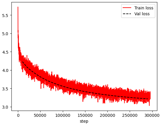
Training and validation loss in Librilight
Generations
Example 1
Example 2
It sounds like the identity is being informed by the prompt, and also the style is mantained. The model seems to be able to generate sometimes some words or ‘word-like’ sounds. The prosody and rhythm of speaking sounds quite coherent too. However the audio quality is not the best as some artifacts can be heard.
Effect of temperature
Next, I explored the effect of temperature but instead of sampling from a set of temperatures, I continuously increased it from 0.01 to 2, so we can listen how speech is heating up.
Example 1
Example 2
Speech Interpolations
Example 1
Example 2
Out of domain prompts
Singing example 1
Singing example 2
Drums
Scratch
Guitar Riff
Moooo
References
- Copet, J., Kreuk, F., Gat, I., Remez, T., Kant, D., Synnaeve, G., … & Défossez, A. (2023). Simple and Controllable Music Generation. arXiv preprint arXiv:2306.05284.
- Défossez, A., Copet, J., Synnaeve, G., & Adi, Y. (2022). High fidelity neural audio compression. arXiv preprint arXiv:2210.13438.
- Oord, A. V. D., Dieleman, S., Zen, H., Simonyan, K., Vinyals, O., Graves, A., … & Kavukcuoglu, K. (2016). Wavenet: A generative model for raw audio. arXiv preprint arXiv:1609.03499.
- Pepino, L., Riera, P., Ferrer, L. (2023). EnCodecMAE: Leveraging neural codecs for universal audio representation learning. arXiv preprint arXiv:2309.07391
- Radford, A., Wu, J., Child, R., Luan, D., Amodei, D., & Sutskever, I. (2019). Language models are unsupervised multitask learners. OpenAI blog, 1(8), 9.
- Wang, C., Chen, S., Wu, Y., Zhang, Z., Zhou, L., Liu, S., … & Wei, F. (2023). Neural codec language models are zero-shot text to speech synthesizers. arXiv preprint arXiv:2301.02111.